Analysis with SPSS/PSPP/JASP
Analysis with SPSS
Why use SPSS? SPSSSPSS statstical software SPSS is one of the most widespread statistical programs and provides automated processes with the help of a very detailed graphical interface and a large number of their configuration. In addition it provides the option of writing code with its help Syntax to speed up repetitive processes.
The following is a typical example of Statistical Data Analysis
Sample description
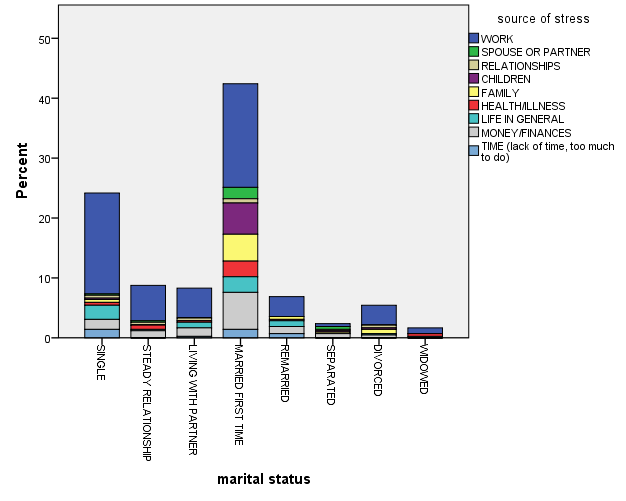
From the composite bar graph of percentages on the whole we observe that
1. Work is the most important stressor in all categories of marital status
2. The general concern for the evolution of life concerns mainly the single, those who got married for the first time and those who live with their parents.
3. The marital status that covers the widest range of sources of stress was presented to single people and married people for the first time.

Chi Square Test2
With the help of the Chi Square test of independence between the variable of marital status and the variables of smoking habits and source of stress we observe that there is marital status and we expect to have different values in whether the research participants smoke as well as to their main source of stress.
|
Chi-Square Tests |
|||
|
Value |
df |
AsymptoticSignificance (2-sided) |
|
| Pearson Chi-Square |
19,059a |
7 |
,008 |
| Likelihood Ratio |
18,338 |
7 |
,011 |
| Linear-by-Linear Association |
,829 |
1 |
,363 |
| N of Valid Cases |
436 |
||
| a. 3 cells (18,8%) have expected count less than 5. The minimum expected count is 1,36. | |||
|
Chi-Square Tests |
|||
|
Value |
df |
AsymptoticSignificance (2-sided) |
|
| Pearson Chi-Square |
112,174a |
56 |
,000 |
| Likelihood Ratio |
119,829 |
56 |
,000 |
| Linear-by-Linear Association |
4,930 |
1 |
,026 |
| N of Valid Cases |
422 |
||
| a. 53 cells (73,6%) have expected count less than 5. The minimum expected count is ,20. | |||
Non parametric correlation
To control the degree of the relationship between the previous variables, a correlation was performed Spearman and the results showed that the main source of stress is to a small extent influenced by the marital status while the smoking habits are not related to the marital status of the respondent.
|
Correlations |
||||
|
marital status |
smoker |
|||
| Spearman’s rho | marital status | Correlation Coefficient |
1,000 |
,073 |
| Sig. (2-tailed) |
. |
,128 |
||
| N |
439 |
436 |
||
| smoker | Correlation Coefficient |
,073 |
1,000 |
|
| Sig. (2-tailed) |
,128 |
. |
||
| N |
436 |
436 |
||
|
Correlations |
||||
|
marital status |
source of stress |
|||
| Spearman’s rho | marital status | Correlation Coefficient |
1,000 |
,156** |
| Sig. (2-tailed) |
. |
,001 |
||
| N |
439 |
422 |
||
| source of stress | Correlation Coefficient |
,156** |
1,000 |
|
| Sig. (2-tailed) |
,001 |
. |
||
| N |
422 |
422 |
||
| **. Correlation is significant at the 0.01 level (2-tailed). | ||||
A minimal effect of Gender on the causes of anxiety was also observed.
|
Correlations |
||||
|
sex |
source of stress |
|||
| Spearman’s rho | sex | Correlation Coefficient |
1,000 |
,099* |
| Sig. (2-tailed) |
. |
,043 |
||
| N |
439 |
422 |
||
| source of stress | Correlation Coefficient |
,099* |
1,000 |
|
| Sig. (2-tailed) |
,043 |
. |
||
| N |
422 |
422 |
||
| *. Correlation is significant at the 0.05 level (2-tailed). | ||||
Two Way ANOVA
Results
|
Tests of Between-Subjects Effects |
|||||
| Dependent Variable: Total negative affect | |||||
| Source |
Type III Sum of Squares |
df |
Mean Square |
F |
Sig. |
| Corrected Model |
1470,276a |
15 |
98,018 |
2,019 |
,013 |
| Intercept |
43267,124 |
1 |
43267,124 |
891,107 |
,000 |
| marital |
658,796 |
7 |
94,114 |
1,938 |
,062 |
| smoke |
32,762 |
1 |
32,762 |
,675 |
,412 |
| marital * smoke |
366,101 |
7 |
52,300 |
0,03 |
,000 |
| Error |
20198,610 |
416 |
48,554 |
||
| Total |
184109,000 |
432 |
|||
| Corrected Total |
21668,887 |
431 |
|||
| a. R Squared = ,068 (Adjusted R Squared = ,034) | |||||
We observe that the interaction between marital status factors and smoking are statistically significant in 0.001 p-level
Further examination of the differences with its help Tukey’s post hoc analysis showed that among other things differences were observed between widows and couples who have a stable relationship.
|
Total negative affect |
|||
| Tukey HSDa,b,c | |||
| marital status |
N |
Subset |
|
|
1 |
2 |
||
| WIDOWED |
7 |
13,14 |
|
| MARRIED FIRST TIME |
186 |
18,35 |
18,35 |
| REMARRIED |
30 |
19,10 |
19,10 |
| DIVORCED |
23 |
19,43 |
19,43 |
| LIVING WITH PARTNER |
36 |
19,56 |
19,56 |
| SINGLE |
103 |
20,20 |
|
| STEADY RELATIONSHIP |
37 |
22,24 |
|
| SEPARATED |
10 |
24,40 |
|
| Sig. |
,066 |
,102 |
|
| Means for groups in homogeneous subsets are displayed.
Based on observed means. The error term is Mean Square(Error) = 48,554. |
|||
| a. Uses Harmonic Mean Sample Size = 20,536. | |||
| b. The group sizes are unequal. The harmonic mean of the group sizes is used. Type I error levels are not guaranteed. | |||
| c. Alpha = 0,05. | |||
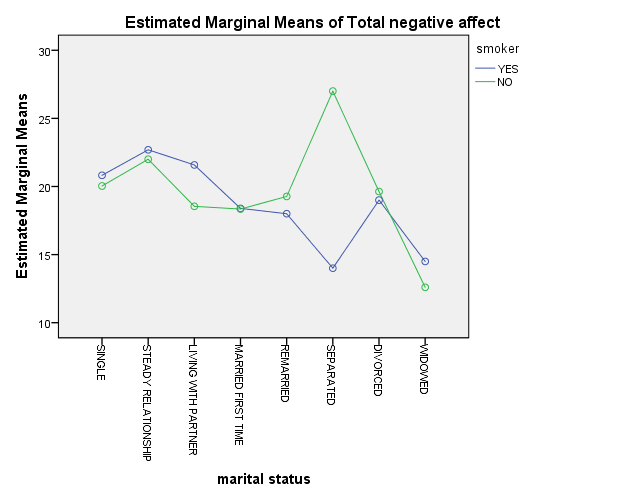
Graph of Interactions
Smoking habits have been shown to affect the values of the rating of negative effects during the transition from an informal relationship to a more formal one (marriage).

3-way ANOVA
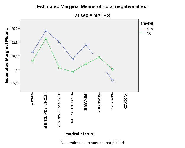
Further examination of the Gender factor in the previous relationship showed that it exhibits statistically significant interactions.
|
Tests of Between-Subjects Effects |
|||||
| Dependent Variable: Total negative affect | |||||
| Source |
Type III Sum of Squares |
df |
Mean Square |
F |
Sig. |
| Corrected Model |
2246,559a |
28 |
80,234 |
1,665 |
,020 |
| Intercept |
44247,737 |
1 |
44247,737 |
918,110 |
,000 |
| marital |
728,713 |
7 |
104,102 |
2,160 |
,037 |
| smoke |
21,755 |
1 |
21,755 |
,451 |
,502 |
| sex |
35,130 |
1 |
35,130 |
,729 |
,394 |
| marital * smoke |
449,449 |
7 |
64,207 |
1,332 |
,233 |
| marital * sex |
347,783 |
6 |
57,964 |
1,203 |
,304 |
| smoke * sex |
79,565 |
1 |
79,565 |
1,651 |
,200 |
| marital * smoke * sex |
75,414 |
5 |
15,083 |
,002 |
,000 |
| Error |
19422,328 |
403 |
48,194 |
||
| Total |
184109,000 |
432 |
|||
| Corrected Total |
21668,887 |
431 |
|||
| a. R Squared = ,104 (Adjusted R Squared = ,041) | |||||
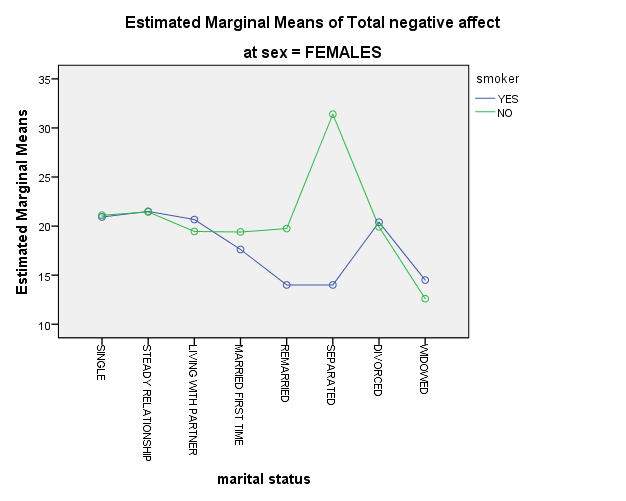
Further graphical examination of our factor showed that no interactions occurred in men while the previous transition we described held true in women.


Conclusion
The difference in the scores of the negative effects during the transition from the free state or the state of informal cohabitation applies only to women.

