Ανάλυση με την βοήθεια του στατιστικού προγράμματος R

Why R? The R program was created as a continuation of an excellent statistical program, S-Plus. It is considered, and not unfairly, to have significant difficulty in handling data and extracting results. However, this difficulty is compensated by the excellent quality graphical results that are fully parameterized and the ready-made libraries that cover all statistical analysis methodologies. It is considered one of the most valuable tools for data analysts worldwide, while this effort is also supported by the many forums of academic and industrial programmers. The program can be downloaded from the website https://www.r-project.org/ and the libraries can be downloaded after installing the program. There are many websites where you can find ready-made code and instructions for use in all analysis methods, while for a first approach that covers almost all modern analysis methods we recommend the book by Venables and Ripley «Modern Applied Statistics with S»

Below is a sample of R's capabilities, while if you want to test it, you can download the code after contacting us.

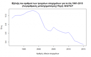
The data concerns the annual number of road accidents for the period 1991 to 2015 and according to ELSTAT

Time Series Analysis

Time series analysis with the help of R contains a significant number of ready-made libraries that automate the processes and cover the entire theory.

Normality Test

In the following graphs we observe a deviation from the normality curve of the data.

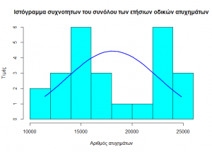
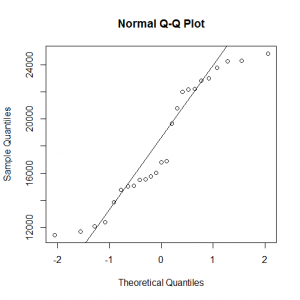
While the Kolmogorov – Smirnov normality test informs us that the data follows the normal distribution at a s.d. of 1%.

One-sample Kolmogorov-Smirnov test

data:  tot

D = 0.16703, p-value = 0.4405

alternative hypothesis: two-sided

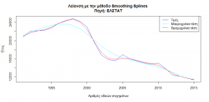
Η συμπεριφορά των οδικών ατυχημάτων δείχνει μια απότομη μείωση κατά την περίοδο 1998 έως και 2004. Η γενική τάση είναι πτωτική και χαρακτηρίζεται από κυκλική συμπεριφορά 10 ετίας 1991 – 2004 και 2005 – 2015.
Η συμπεριφορά αυτή γίνεται περισσότερο κατανοητή και με την βοήθεια του παρακάτω γραφήματος.

Smoothing the time series, i.e. finding the individual trends that affect it, shows a stable short-term trend without individual fluctuations or cyclical repetitions and the downward linear trend after 2015.

A common technique for reducing the order of magnitude of the series values ​​is to transform the values ​​using the logarithmic transformation. Reasons for this type of transformation are to smooth the behavior of the time series and to compare between series with different values.

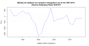
The elimination of the trend is achieved with the first differences, that is, the difference of the next minus the previous value. In the graph of the first differences we observe that the trend has been eliminated and that the data moves around a value close to 0.

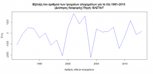
The previous approach has not brought the desired result of eliminating the trend as both individual and overall trends are observed. The second differences do not seem to have the expected image of a constant movement of the data around a value.

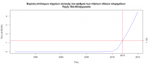
Finding points of abrupt changes in the series 

Finding the points at which the time series has made a sufficient number of changes in its values ​​to give a sign that its cumulative value is changing is presented in the graph below, from which we see that the year in which the data change behavior is 2012.

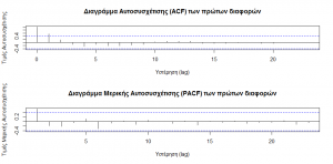
The plot of ACF autocorrelations and partial PACF autocorrelations shows that an appropriate model for this time series is ARIMA(0,1,1)

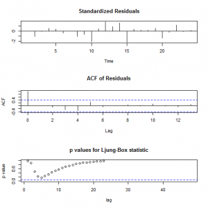
The diagnostics of this model show that

1.The residuals follow the normal distribution

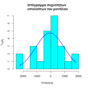
Which is also confirmed by the Shapiro – Wilk test

Shapiro-Wilk normality test

data:  fit1$resid

W = 0.96244, p-value = 0.4893

2.Τα υπόλοιπα δεν σχηματίζουν μια αυτοπαλίνδρομη χρονική σειρά (ACF of Residuals) και σύμφωνα με το Ljung – Box – Pierce Statistic το μοντέλο κρίνεται επαρκές.

A possible candidate model that could describe this time is described by the equation Ŷ_t   =  μ  + Y_t-1   – θ₁e_t-1 

and by replacing the numerical coefficients it becomes

Ŷ_t   =  -388.5 + Y_t-1  +0.014e_t-1 

The model presents significant disadvantages such as the strong influence of the average value (constant) which forces the coefficient to take a positive value.

Conclusion

The model needs review and possible removal of the constant term for safe predictions.