

STATA is owned by StataCorp LLC and its main advantage is the freedom it provides to the user through continuous growing and evolving libraries provided by the company and users through various sites or blogs such as. The Stata blog. Although the main advantage of the program is its code, some users may find it difficult to write the code and manipulate the results.
With a simple example we will try to show some of the capabilities of the program through time series analysis. We used the GDP index dataset for the years 1995 to 2017 from ELSTAT .
Import dataset command
import excel «C:\…\stata_example.xlsx», sheet(«Φύλλο1») firstrow
| year | pop | GDP |
| 1995 | 10562164 | 8811.0354 |
| 1996 | 10608821 | 9712.3557 |
| 1997 | 10661312 | 10759.669 |
| 1998 | 10720566 | 11684.323 |
| 1999 | 10761705 | 12431.927 |
| 2000 | 10805796 | 13071.436 |
| 2001 | 10862146 | 14011.397 |
| 2002 | 10902005 | 14993.642 |
| 2003 | 10928091 | 16371.103 |
| 2004 | 10955163 | 17682.605 |
| 2005 | 10987352 | 18133.788 |
| 2006 | 11020393 | 19768.947 |
| 2007 | 11048499 | 21061.195 |
| 2008 | 11077863 | 21844.501 |
| 2009 | 11107024 | 21385.943 |
| 2010 | 11121383 | 20324.041 |
| 2011 | 11104995 | 18642.861 |
| 2012 | 11045040 | 17311.292 |
| 2013 | 10965241 | 16475.176 |
| 2014 | 10892369 | 16401.986 |
| 2015 | 10820964 | 16381.013 |
| 2016 | 10775989 | 16377.889 |
| 2017 | 10768193 | 16736.104 |
Descriptives
label variable year «Year»
label variable pop «Population»
label variable GDP «GDP»
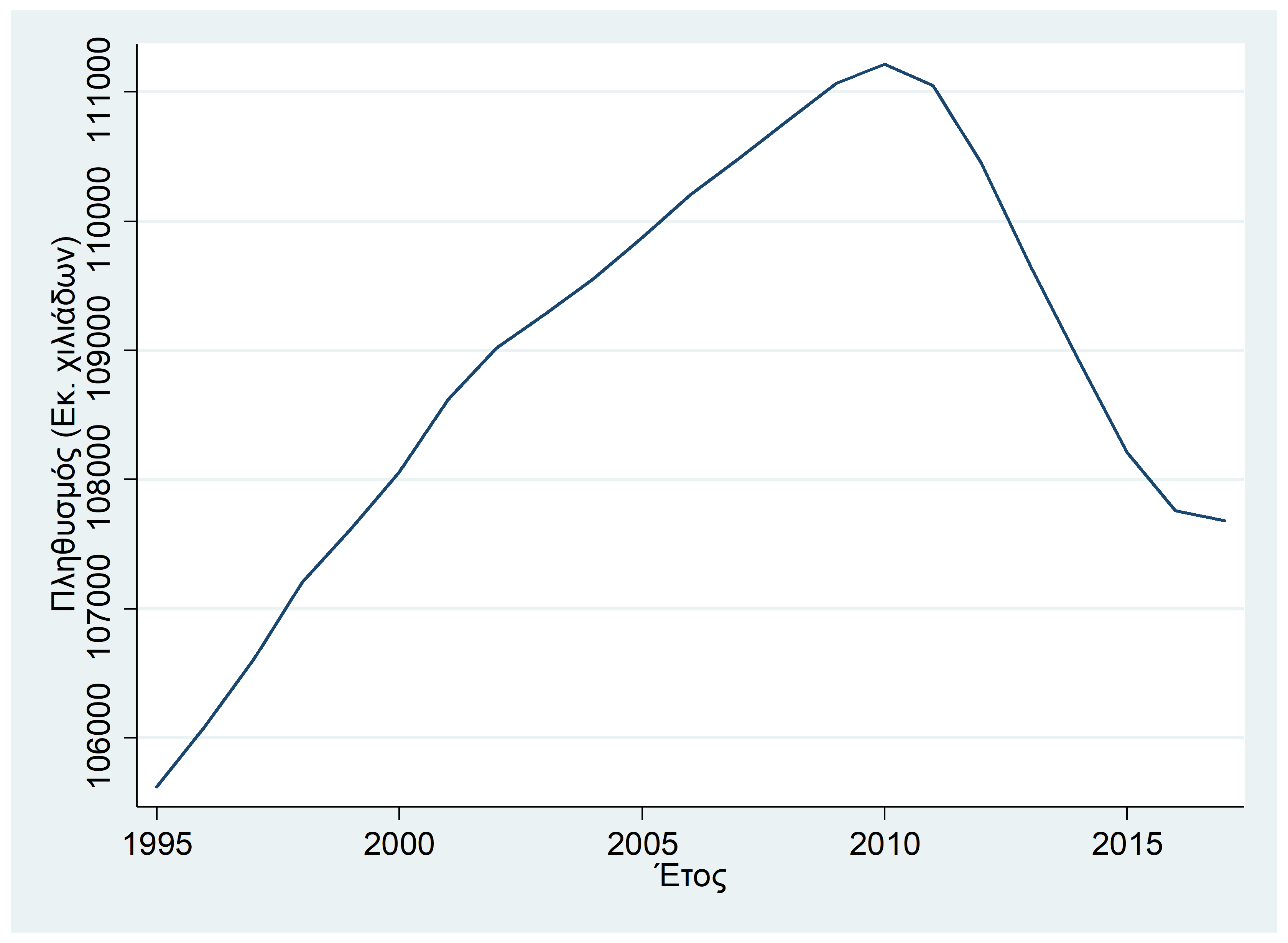
Για την καλύτερη γραφική απεικόνιση των δεδομένων κατασκευάσαμε μια νέα μεταβλητή, την pop2
generate pop2=pop/100
label pop2 «Πληθυσμός (Εκατοντάδες)»
The population change time diagram is generated by the tsline pop2 command and produces the following graph
Similarly, command tsline GDP produces the below graph
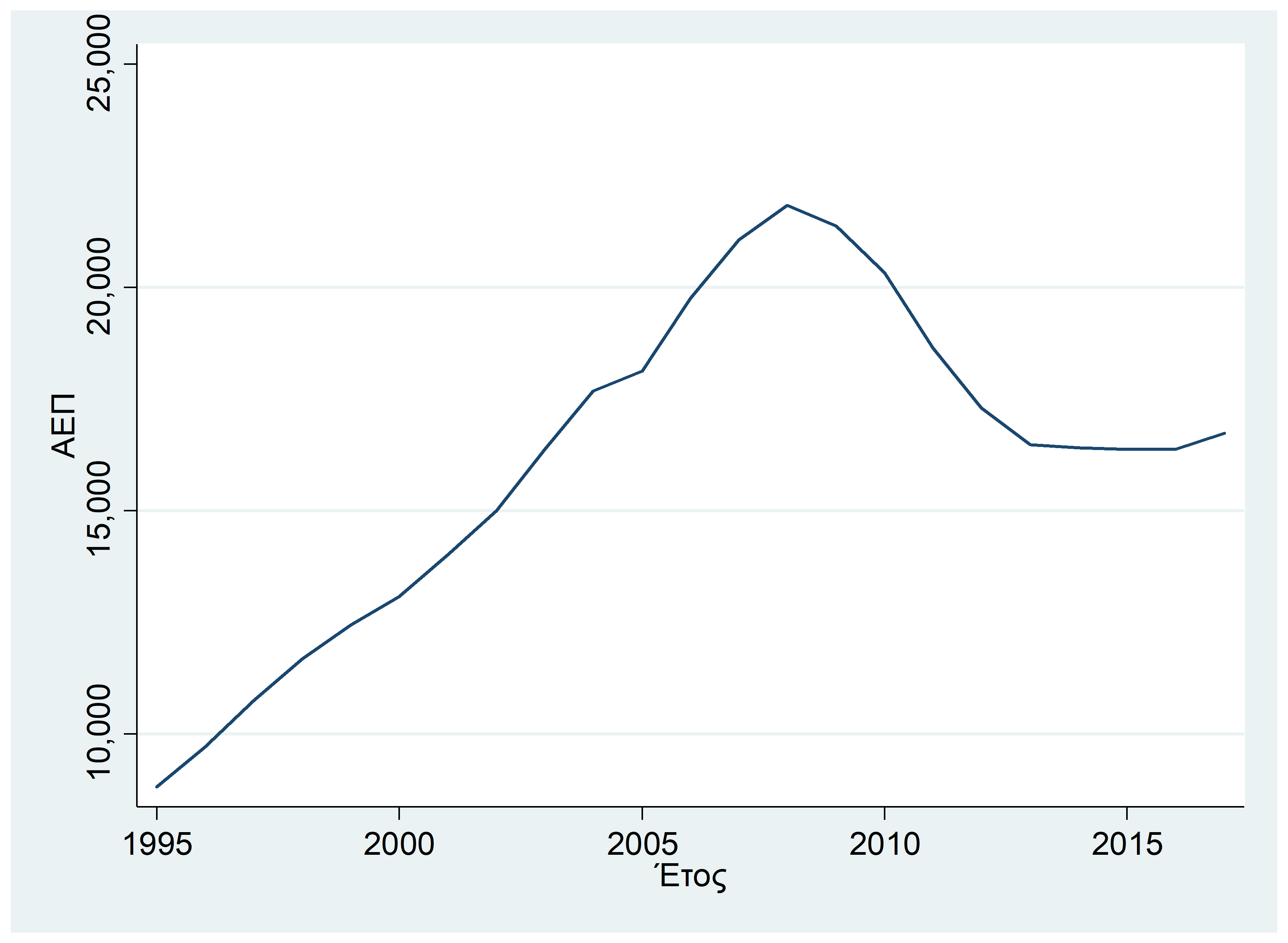
We observe a similar change of the two sizes characterized by the steady decline in their prices after 2010.
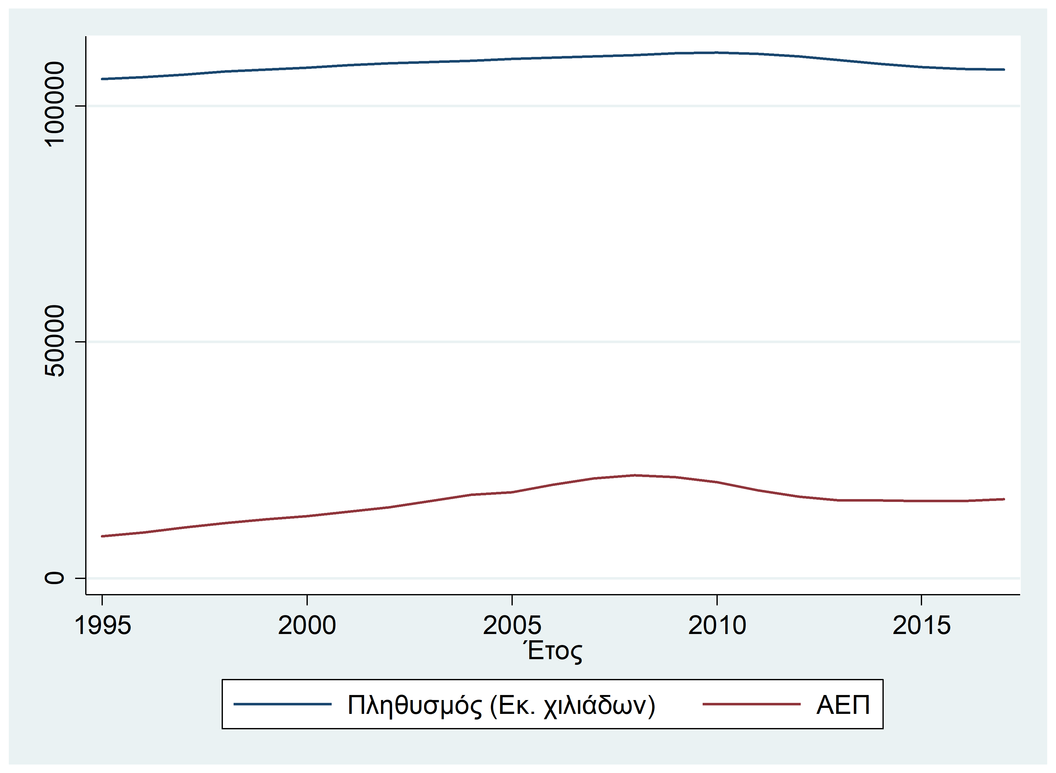
Finally, the simultaneous representation of the two variables with the help of the tsline GDP pop2 command can not render in detail the time changes.
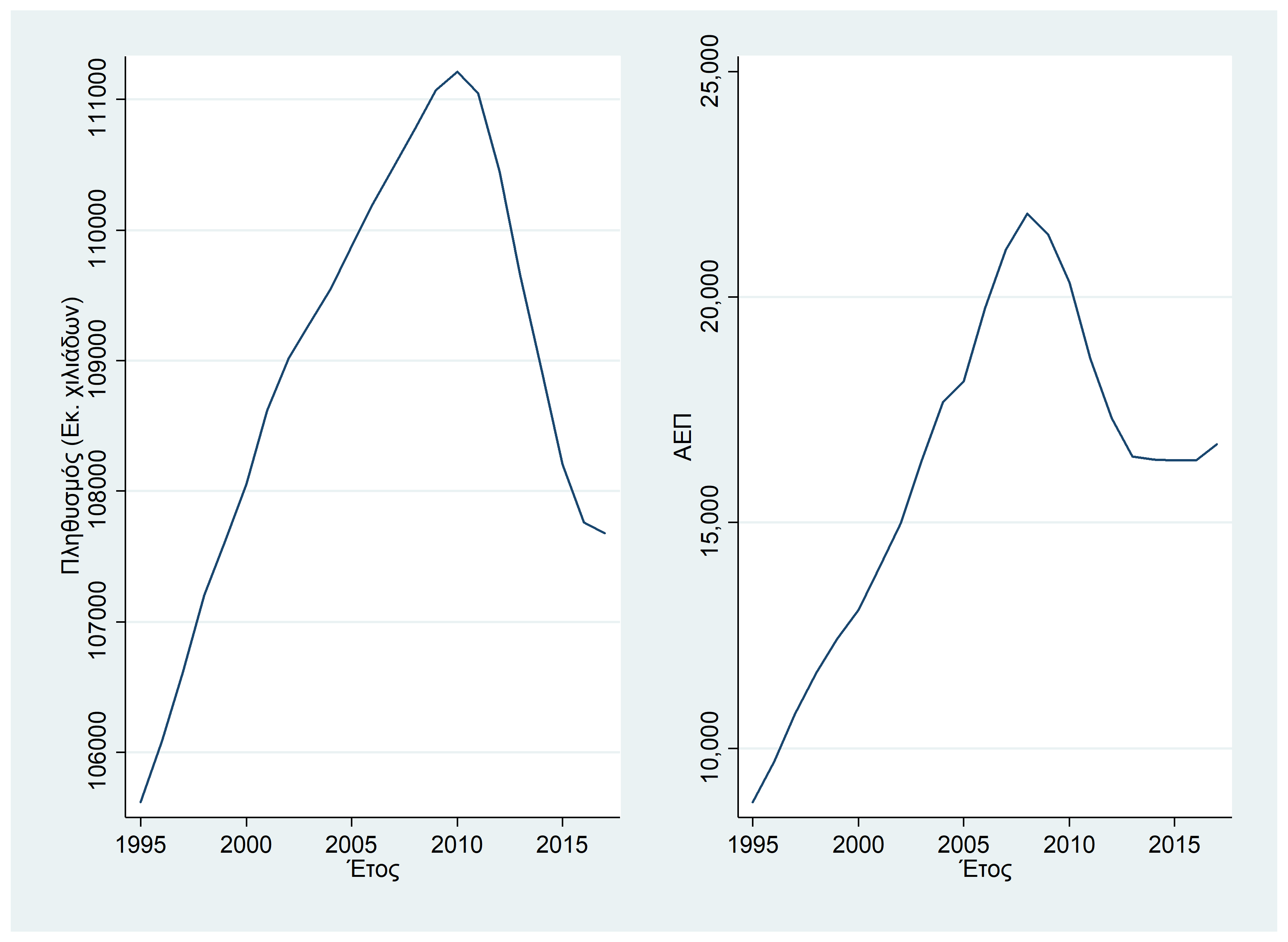
One solution is to combine these two graphs with the help of commands
line pop2 year, saving(g1)
line GDP year, saving(g2)
gr combine g1.gph g2.gph
The first test was performed with the help of a linear regression model with the help of the command
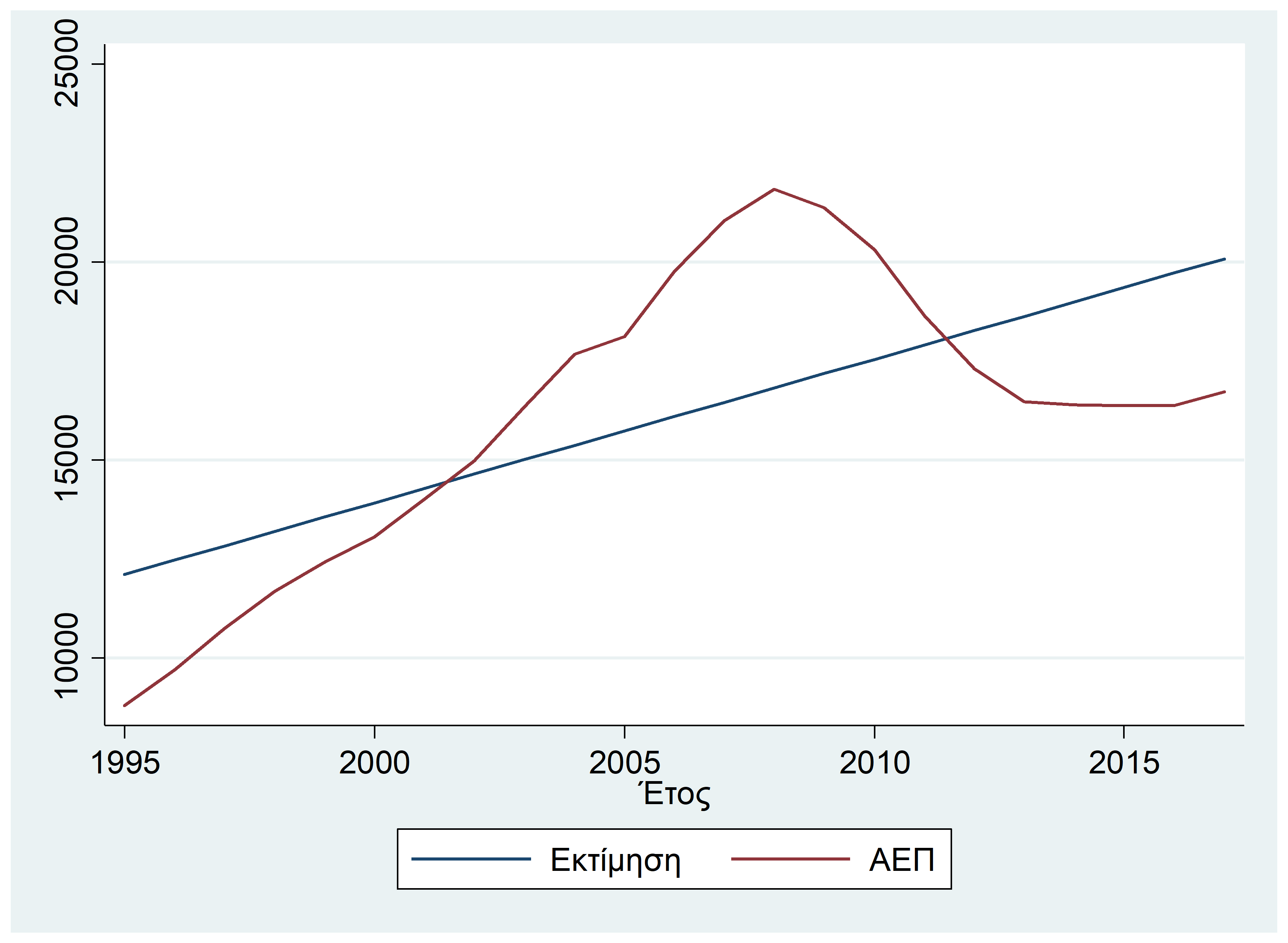
regress GDP year
and the results showed that the model is statistically significant (F (1.21) = 16.45, p <0.001) and of moderate interpretability (R2=43.93)
The comparison of real versus estimated values with the help of commands
predict fitted_values
line fitted_values GDP year
shows that linear regression can not capture changes in GDP
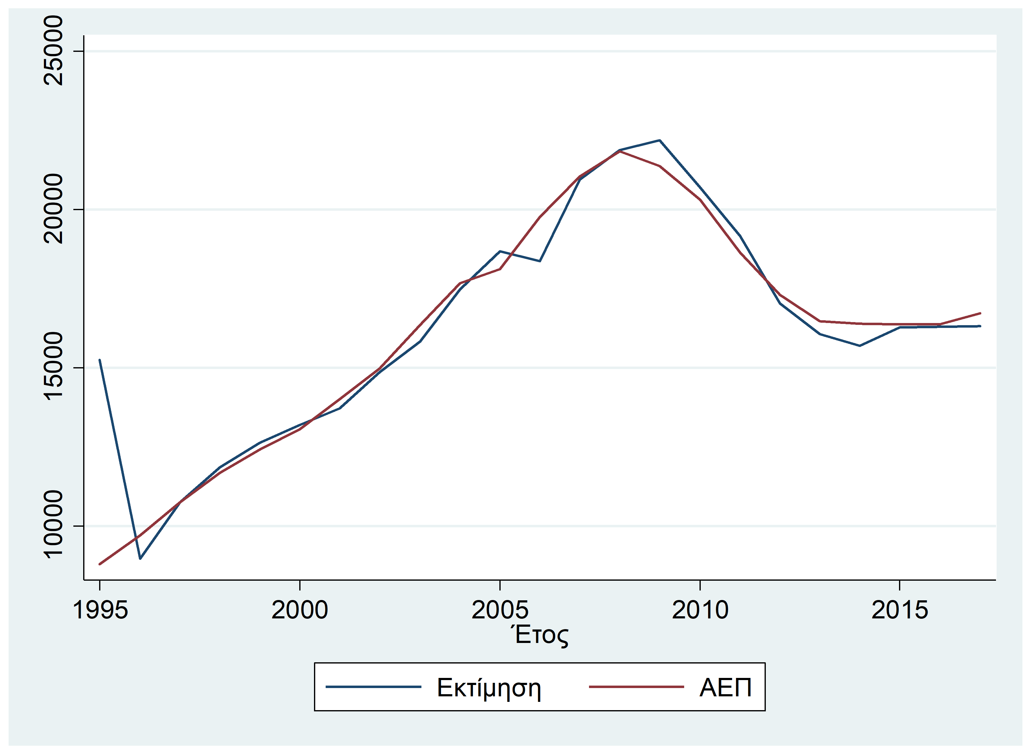
The second estimate was made using the ARIMA method (p, d, q) and led to the ARMA model (2.0) as it presented the lowest BIC and AIC coefficient. The new assessment was made with the help of the commands
arima GDP, arima(2,0,0)
predict f1
estout, stat(aic bic)
line f1 GDP year
was clearly improved as shown in the graph below
This was a simple example of using STATA for analysis. For any question or if you need help with your analysis you can contact us.